PyTorch, a popular deep learning library, provides powerful tools for building neural networks. In this article, we will explore the building blocks of PyTorch and demonstrate the progression from a simple logistic regression model to a multi-layer perceptron (MLP) capable of tackling nonlinear classification problems.
As we've seen in other articles, PyTorch tensors are the core of the neural networks as they can store a history of the operations that have been performed. By combining tensors and operations, we can construct dynamic computational graphs that represent neural networks.By combining tensors and operations, we can construct dynamic computational graphs that represent neural networks. By combining tensors and operations, we can construct dynamic computational graphs that represent neural networks.
This Article will cover a bit of understanding of nn module in PyTorch, how to create a basic neural network with a logistic regresion behaviuor and some introspection of the neural network
Logistic Regression: A Linear Classifier
To illustrate the limitations of logistic regression, we will begin with a simple 2D binary classification problem. In this problem, the classes are linearly separable, and we can visualize the decision boundary between them.
Let's start by generating a dataset consisting of half-moon shapes:
      np.random.seed(0)
      num_samples = 300

      X, y = sklearn.datasets.make_moons(num_samples, noise=0.20)
The make_moons function from the sklearn.datasets module generates a dataset of half-moon shapes with a specified number of samples and added noise. Next, we split the dataset into training, validation, and test sets:
      X_tr = X[:100].astype('float32')
      X_val = X[100:200].astype('float32')
      X_te = X[200:].astype('float32')

      y_tr = y[:100].astype('int32')
      y_val = y[100:200].astype('int32')
      y_te = y[200:].astype('int32')
We use the first 100 samples for training, the next 100 for validation, and the remaining samples for testing. The labels are encoded as integers.
To visualize the dataset, we can plot the training examples:
plt.scatter(X_tr[:, 0], X_tr[:, 1], s=40, c=y_tr, cmap=plt.cm.Spectral)
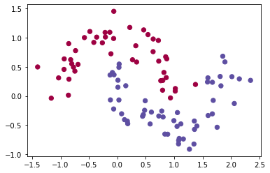
The scatter plot displays the points in the 2D feature space, with different colors representing the two classes.
Logistic Regression vs. Multi-layer Perceptrons
We will now demonstrate the limitations of logistic regression in handling nonlinear classification problems. Logistic regression is a linear classifier, meaning it can only separate classes using linear decision boundaries. In contrast, MLPs can handle nonlinear problems by introducing nonlinear activation functions and hidden layers.
At the heart of neural networks lie layers, and the simplest type of layer is a fully-connected layer, also known as a dense feed forward layer. Mathematically, a fully-connected layer can be expressed as:
Here, $x$ represents the input vector, $y$ is the output vector, $W$ and $b$ are the weights and biases respectively (represented as a matrix and a vector), and $g$ denotes the activation function. Each element of the input vector contributes to every element of the output vector, giving rise to the term "dense". The layer processes each input independently in a feed forward manner, making it acyclical.
\( y = g(W^{\top} x + b) \)Setting up the Network:
To begin, we define a class called "Net" that inherits from the PyTorch class "nn.Module." This class will serve as the blueprint for our neural network. Inside the class, we initialize the network's variables, which are the weights that can be updated during the training process.
In our example, we are creating a logistic regression network with two input units (num_features) and two output units (num_output). The weights of the first layer are defined as W_1 [2, 2] and b_1 [2]. The shape of the weight matrix is determined by the number of units going out and the number of units going in.
First layer
The first layer of our network consists of the weight matrix W_1 and the bias vector b_1. We use PyTorch's "nn.Parameter" to define these variables as learnable parameters of the network. The weight matrix W_1 is initialized with random values using "torch.randn" function, and the bias vector b_1 is also initialized randomly.
Forward Function
Forward Function: The "forward" function defines the forward pass of the neural network. It describes the flow of data through the network's layers. In our case, we start by applying a linear transformation to the input data using the weights and biases of the first layer. This is done by calling the "F.linear" function, passing in the input data (x), the weight matrix (self.W_1), and the bias vector (self.b_1). The result is stored in the variable "x."
Finally, we apply the softmax function to the output "x" along the second dimension (dim=1) using PyTorch's "F.softmax" function. This converts the output into probabilities, making it suitable for multi-class classification problems.
Initializing the Network
To create an instance of our neural network, we simply instantiate the "Net" class and assign it to the variable "net." This initializes the weights and biases of the network.
      class Net(nn.Module):

          def __init__(self):
              super(Net, self).__init__()
              # first layer
              self.W_1 = nn.Parameter(torch.randn(num_output, num_features))
              self.b_1 = nn.Parameter(torch.randn(num_output))

          def forward(self, x):
              x = F.linear(x, self.W_1, self.b_1)

              return F.softmax(x, dim=1) # softmax to be performed on the second dimension

      net = Net()
For those who are not that familiar with python syntaxis, the line of code
super(Net, self).__init__() is calling the constructor of the parent class
nn.Module from which the Net class inherits.
In Python, when a class inherits from another class, the child class can
override the methods and attributes of the parent class. However, sometimes
it's necessary to also initialize the attributes and behavior of the parent
class before adding or modifying anything in the child class.
In this case, super(Net, self) refers to the parent class nn.Module,
and __init__() is the constructor method of nn.Module. By calling
super(Net, self).__init__() , we ensure that the initialization
process of the parent class is executed before adding any additional
initialization steps specific to the Net class.
This line of code is essential for proper initialization and inheritance,
allowing the Net class to inherit the behavior and attributes from nn.Module
and initialize them before adding its own specific attributes and behavior.
Exploring the Parameters of the Neural Network
Once we have defined our neural network net, it is essential to understand and explore its parameters. Parameters are the learnable weights and biases that the network updates during the training process. In this section, we will examine the parameters of our network and gain insights into their values, sizes, and gradients.
Listing Named Parameters
To begin, let's list all the named parameters in our network. The named_parameters() method provides us with the names and values of each parameter. Let's take a look:
      print("NAMED PARAMETERS")
      print(list(net.named_parameters()))
      print()
The output will display the names and corresponding values of the parameters:
      NAMED PARAMETERS
      [('W_1', Parameter containing:
      tensor([[-0.7289,  2.0885],
              [-0.7081, -0.0942]], requires_grad=True)), ('b_1', Parameter containing:
      tensor([-0.3124, -0.0223], requires_grad=True))]
In our case, the named parameters are W_1 and b_1. The values of these parameters are also shown along with the information that they require gradient computation (requires_grad=True).
Listing parameters
Next, we can list all the parameters in the network using the parameters() method. This method returns a list of tensors without their names. Let's see it in action:
      print("PARAMETERS")
      print(list(net.parameters()))
      print()
The output will provide the tensor values of the parameters:
      PARAMETERS
      [Parameter containing:
      tensor([[-0.7289,  2.0885],
              [-0.7081, -0.0942]], requires_grad=True), Parameter containing:
      tensor([-0.3124, -0.0223], requires_grad=True)]
We can observe that the tensor values are the same as in the named parameters.
Accessing Individual Parameters
It is also possible to access individual parameters directly by treating them as attributes of the network. Let's examine the weights and biases of the first layer, W_1 and b_1, respectively:
      print('WEIGHTS')
      print(net.W_1)
      print(net.W_1.size())
      print('\nBIAS')
      print(net.b_1)
      print(net.b_1.size())
By running this code, we obtain the following output:
      WEIGHTS
      Parameter containing:
      tensor([[-0.7289,  2.0885],
              [-0.7081, -0.0942]], requires_grad=True)
      torch.Size([2, 2])

      BIAS
      Parameter containing:
      tensor([-0.3124, -0.0223], requires_grad=True)
      torch.Size([2])
We can see that net.W_1 represents the weight matrix of the first layer, and net.b_1 represents the bias vector. The sizes of these tensors are also provided.
Exploring a Specific Parameter
To delve deeper into a particular parameter, let's focus on net.W_1. We will examine its tensor data, gradient, and whether it is considered a leaf in the computational graph. Consider the following code snippets:
      WEIGHTS
      Parameter containing:
      tensor([[-0.7289,  2.0885],
              [-0.7081, -0.0942]], requires_grad=True)
      torch.Size([2, 2])

      BIAS
      Parameter containing:
      tensor([-0.3124, -0.0223], requires_grad=True)
      torch.Size([2])
Testing the Network: Forward Pass and Gradients
Once we have constructed our network, we can easily utilize it by invoking its graph and running a forward pass. The code below below demonstrates an example of how to execute the forward pass of our network:
      X = torch.randn(5, num_features)
      print('input')
      print(X)

      print('\noutput')
      print(net(X))
The output will be:
      input
      tensor([[ 0.8958, -0.0290],
              [ 0.8017, -0.5530],
              [-0.3895,  1.6482],
              [ 0.2550, -1.1994],
              [ 0.2616, -0.5097]])

      output
      tensor([[0.4080, 0.5920],
              [0.1804, 0.8196],
              [0.9650, 0.0350],
              [0.0515, 0.9485],
              [0.1965, 0.8035]], grad_fn=< SoftmaxBackward0>)
The torch.randn function generates a random tensor of shape
(5, num_features) to serve as the input for the network. By passing
this tensor to net(X), we obtain the output of the network. The
resulting tensor is printed, revealing the network's prediction for each input
sample.
Next, let's examine the gradients of the network parameters. Gradients provide
crucial information about the sensitivity of the network's output to changes
in its parameters. The code snippet below demonstrates how to inspect the
gradients:
      for p in net.parameters():
          print(p.data)
          print(p.grad)
          print()
The output will be:
      tensor([[-0.7289,  2.0885],
        [-0.7081, -0.0942]])
      None

      tensor([-0.3124, -0.0223])
      None
Here, we iterate over the network's parameters using a for loop. For
each parameter p, we print both the data (the current parameter values)
and the gradient (the derivative of the loss function with respect to the
parameter). However, when printing the gradients, we observe
None values. This is because we have not yet computed any gradients.
To compute gradients, we need to perform a backward pass through the network.
The code below demonstrates how to perform the backward pass and compute
gradients for a specific input:
      X = torch.randn(7, num_features)
      out = net(X)
      out.backward(torch.randn(7, num_output))
In this example, we generate a random tensor X with a shape of
(7, num_features) as the input. We then pass this input through the
network using net(X), and finally, we call backward on the output
tensor out. The backward function calculates the gradients using automatic
differentiation.
After computing the gradients, we can once again inspect them:
      for p in net.parameters():
      print(p.data)
      print(p.grad)
      print()
The outout will be:
      tensor([[-0.7289,  2.0885],
        [-0.7081, -0.0942]])
      tensor([[ 0.4015, -0.0854],
              [-0.4015,  0.0854]])

      tensor([-0.3124, -0.0223])
      tensor([-0.8066,  0.8066])
This time, we observe non-zero gradients, indicating that the backward pass
successfully computed the gradients for each parameter.
Finally, to zero the accumulated gradients, we use the
zero_grad function provided by PyTorch. The snippet below demonstrates
how to zero the gradients:
      net.zero_grad()
      for p in net.parameters():
          print(p.data)
          print(p.grad)
The outout will be:
      tensor([[-0.7289,  2.0885],
        [-0.7081, -0.0942]])
      tensor([[0., 0.],
              [0., 0.]])
      tensor([-0.3124, -0.0223])
      tensor([0., 0.])
By calling zero_grad, we reset all the gradients of the network
parameters to zero. This is a necessary step before performing the next
backward pass, as it ensures that the new gradients are computed independently
from the previous gradients.
By understanding the process of running a forward pass, computing gradients,
and zeroing the gradients, we gain valuable insights into the inner workings
of our network. These steps are fundamental to training neural networks, and
PyTorch provides an efficient and intuitive interface to perform these
operations.
In this article, we explored the implementation and testing of a neural network using PyTorch. We learned how to construct a network by defining its architecture and forward pass, and we saw how to examine gradients and zero them for subsequent computations. These steps provide us with a solid foundation for understanding the inner workings of a neural network. In the next post, we will delve into the exciting topic of training a neural network. We will explore how to optimize the network's parameters using techniques such as backpropagation and gradient descent, enabling our network to learn and make accurate predictions. Stay tuned for an in-depth exploration of the training process and its significance in neural network applications.