Training Neural Networks

In this article, we dive into the essential components of training a neural network: the loss function, optimizer, and accuracy measure. These elements play a crucial role in guiding the network towards optimal performance. Let's explore each of them in detail.

Loss Function

The loss function quantifies the discrepancy between the predicted output of the neural network and the true labels. A commonly used loss function for classification tasks is cross-entropy loss. It measures the dissimilarity between the predicted probabilities (ys) and the target probabilities (ts). The cross-entropy loss is computed per sample and then averaged over all samples. In a future post we'll se how to define it mathematically, In the mean time you will have to trust me in this one. The Loss function implementation is:

    
      def cross_entropy(ys, ts):
          cross_entropy = -torch.sum(ts * torch.log(ys), dim=1, keepdim=False)
          return torch.mean(cross_entropy)
    
  

As a key concepts here we should understand that the use of logarithm and the negative sign in the cross-entropy loss calculation serves specific purposes in the context of classification tasks. Let's understand their significance:

Logarithm (torch.log()): In the cross-entropy loss formula, we need to compute the logarithm of the predicted values (ys). This is because the cross-entropy loss is derived from the concept of information theory, where the logarithm helps in measuring the "information content" or "surprise" associated with each prediction. Taking the logarithm allows us to magnify the loss for incorrect predictions and penalize them more heavily.

Negative sign (-): The negative sign is applied to the sum of the element-wise multiplication of the target values (ts) and the logarithm of the predicted values (ys). In the context of gradient-based optimization algorithms, such as stochastic gradient descent (SGD), the goal is to minimize the loss function. The optimization algorithms work by iteratively updating the model parameters in the direction that reduces the loss.
By negating the sum in the cross-entropy loss calculation, we convert the objective from maximizing the likelihood (as in the case of maximum likelihood estimation) to minimizing the loss. Minimizing the loss is often computationally easier and more stable than maximizing it. It allows us to leverage the existing optimization algorithms that are designed for minimization.
Additionally, the negative sign ensures that the loss value increases as the predicted probabilities deviate further from the target probabilities. This aligns with the goal of penalizing incorrect predictions and encourages the model to adjust its parameters in a way that improves its predictions.
In summary, the negative sign in the cross-entropy loss simplifies the computational optimization process and aligns with the goal of minimizing the loss to improve the model's predictions.

Optimizer

To update the network's parameters and minimize the loss function, we employ an optimizer. In this case, we use Stochastic Gradient Descent (SGD). The optimizer computes the gradients of the loss function with respect to all parameters in the network and updates them accordingly. The learning rate (lr) determines the step size of the parameter updates.

    
      import torch.optim as optim

      optimizer = optim.SGD(net.parameters(), lr=0.01)
    
  

Bare in mind that PyTorch offers a variety of optimizers that can be used to train neural networks. Each optimizer employs a different update rule for adjusting the network's parameters based on the computed gradients. The choice of optimizer depends on the specific characteristics of the task and the network architecture. Here are some commonly used optimizers in PyTorch:

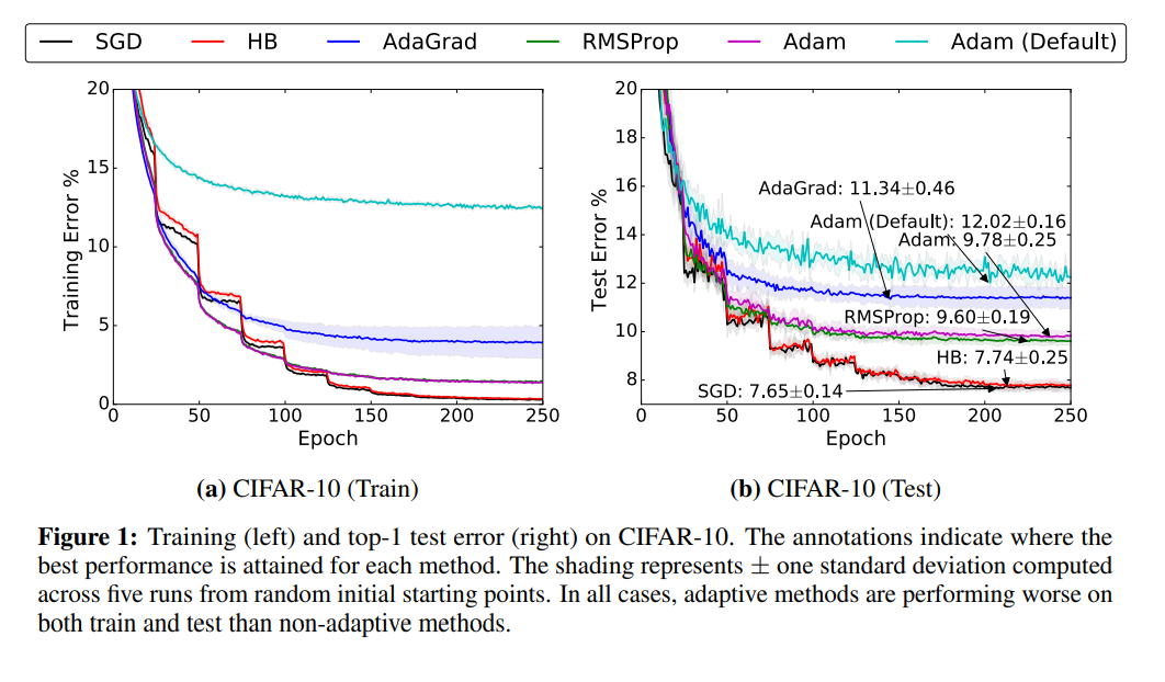
1. Stochastic Gradient Descent (SGD):SGD is a basic optimization algorithm that updates the parameters in the opposite direction of the gradients. It takes a fixed learning rate and can suffer from slow convergence or getting stuck in local minima. However, it is computationally efficient and can work well with large-scale datasets.
2. Adam:Adam (Adaptive Moment Estimation) is an extension of SGD that adapts the learning rate for each parameter based on the estimates of the first and second moments of the gradients. It combines the benefits of both AdaGrad and RMSprop optimizers. Adam is known for its robustness, fast convergence, and good performance across a wide range of tasks.
3. RMSprop:RMSprop is an optimizer that divides the learning rate by an exponentially decaying average of squared gradients. It helps in adjusting the learning rate dynamically for each parameter, allowing faster convergence. RMSprop is particularly useful in scenarios where the gradients exhibit large variations.
4. Adagrad:Adagrad adapts the learning rate for each parameter by scaling it inversely proportional to the sum of the historical squared gradients. It performs larger updates for infrequent parameters and smaller updates for frequent parameters. Adagrad is beneficial when dealing with sparse data or when the learning rate needs to be automatically adjusted.
5. Adadelta:Adadelta is an extension of Adagrad that improves its limitations by addressing the problem of diminishing learning rates. Instead of accumulating all past squared gradients, Adadelta maintains a running average of gradients and updates the parameters based on the ratio of the current update to the running average of past updates. It is particularly effective when dealing with recurrent neural networks (RNNs).
6. AdamW:AdamW is a variant of the Adam optimizer that incorporates weight decay regularization during the parameter updates. It helps prevent overfitting by adding an additional term to the loss function that penalizes large weights.

The choice of the optimizer depends on the specific task, the architecture of the neural network, and the characteristics of the dataset. There is no single "best" optimizer that suits all scenarios. It is often recommended to experiment with different optimizers and learning rates to find the one that yields the best performance for a particular task. Additionally, advanced optimization techniques like learning rate scheduling and warm-up steps can also be employed to further improve convergence and performance.
This is a very extensive topic, in future posts we'll compare the performance of various optimizers and see the benefits in first hand.

Accuracy

To assess the performance of the neural network, we need a metric that measures how well it predicts the correct labels. Accuracy is a commonly used evaluation metric for classification tasks. It calculates the proportion of correct predictions over a batch of samples. The accuracy function can be defined as follows:

    
      def accuracy(ys, ts):
          correct_prediction = torch.eq(torch.max(ys, 1)[1], torch.max(ts, 1)[1])
          return torch.mean(correct_prediction.float())
    
  

[1]: Wilson, A. C., Roelofs, R., Stern, M., Srebro, N., & Recht, B. (2017). The marginal value of adaptive gradient methods in machine learning. Advances in neural information processing systems, 30.