In PyTorch, the autograd package plays a central role in all neural networks. It provides automatic differentiation for tensor operations, enabling efficient computation of gradients. This article will delve into the concept of automatic differentiation and its implementation in PyTorch, highlighting the power and flexibility it offers in training neural networks.
Tensor: The Building Block
At the heart of the autograd package lies the torch.Tensor class. When a tensor's attribute .requires_grad is set to True, it becomes capable of "recording" all the operations performed on it. This enables the tensor to track the computation graph, which in turn allows for automatic computation of gradients.
To illustrate this, let's consider a simple example:
      import torch
      x = torch.ones(2, 2, requires_grad=True)
      print(x)
The output will be:
      tensor([[1., 1.],
        [1., 1.]], requires_grad=True)
We can clearly see that we have a "new" attribute asociated to our tensor. By setting requires_grad=True, we inform the tensor x to keep track of the operations applied to it.
Computation Graph and Functions
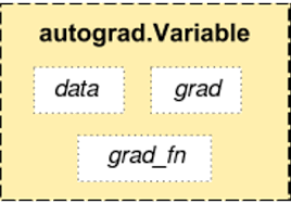
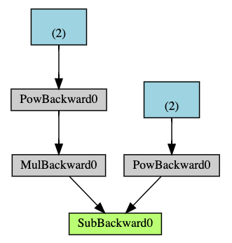
In the autograd framework, tensors and functions are intricately connected, forming an acyclic graph that encodes the complete computation history. Each tensor has a .grad_fn attribute that references the function responsible for creating that tensor (except for tensors created by the user, which have None as their grad_fn).
Let's perform some operations on our tensor x:
      y = x + 2
      print(y)
The output will be:
      tensor([[3., 3.],
        [3., 3.]], grad_fn=< AddBackward0 >)
The tensor y is created as a result of the operation x + 2, and it retains information about the operation through its grad_fn attribute.
brTracking Operations and Gradients
We can continue performing more operations on y:
      z = y * y * 3
      out = z.mean()

      print(z)
      print(out)
The output will be:
      tensor([[27., 27.],
        [27., 27.]], grad_fn=< MulBackward0 >)
      tensor(27., grad_fn=< MeanBackward0 >)
Here, we compute z as the result of y * y * 3, and out as the mean of z. The tensors z and out retain the computation history through their respective grad_fn attributes.
Computing Gradients
To compute the gradients for the tensors involved in the computation graph, we can simply call .backward() on the output tensor. If the tensor is a scalar (contains a single element), no additional arguments are required. However, if the tensor has multiple elements, we need to specify a gradient argument, which is a tensor of matching shape.
By calling .backward() on out, the gradients with respect to x will be computed automatically, d(out)/dx:
      out.backward()
      print(x.grad)
The output will be:
      tensor([[4.5000, 4.5000],
        [4.5000, 4.5000]])
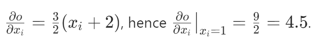
The x.grad tensor contains the gradients of out with respect to x, which are computed as 4.5 in this case.
If we break the math operation. Let's denote the tensor out with o
We have:
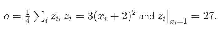
Therefore
Flexibility and Define-by-Run Paradigm
The beauty of the autograd package lies in its flexibility and the
define-by-run paradigm.
Unlike other frameworks that use define-and-run approaches, PyTorch allows you
to define your neural network model dynamically as you execute the code. This
dynamic nature offers several advantages and opens up possibilities for
advanced functionalities in deep learning.
Let's try to perform a few more operations to get used to the syntaxis.
- Define a tensor and set requires_grad to True.
- Multiply the tensor by 2 and assign the result to a new python variable.
- Sum the variable's elements and assign to a new python variable.
- Print the gradients of all the variables.
- Now perform a backward pass on the last variable (NOTE: for each new python variable that you define, call .retain_grad()).
- Print all gradients again.
      x2 = torch.ones(5,5, requires_grad = True)
      y2 = x2 + 2
      g2 = y2*2
      z2 = y2.sum()

      print(x2, x2.grad)
      print(y2, y2.grad)
      print(g2, g2.grad)
      print(z2, z2.grad)
Here, we can see that all the gradients created from the base gradient will have a gradient and will start tracking all the operations.
      tensor([[1., 1., 1., 1., 1.],
         [1., 1., 1., 1., 1.],
         [1., 1., 1., 1., 1.],
         [1., 1., 1., 1., 1.],
         [1., 1., 1., 1., 1.]], requires_grad=True),  None

      tensor([[3., 3., 3., 3., 3.],
         [3., 3., 3., 3., 3.],
         [3., 3., 3., 3., 3.],
         [3., 3., 3., 3., 3.],
         [3., 3., 3., 3., 3.]], grad_fn =< AddBackward0 >), None

      tensor([[6., 6., 6., 6., 6.],
         [6., 6., 6., 6., 6.],
         [6., 6., 6., 6., 6.],
         [6., 6., 6., 6., 6.],
         [6., 6., 6., 6., 6.]], grad_fn=<  MulBackward0 >), None

      tensor(75., grad_fn=< SumBackward0>), None
      z2.backward()

      print(x2.grad)
      print(y2.grad)
      print(g2.grad)
      print(z2.grad)
      tensor([[1., 1., 1., 1., 1.],
        [1., 1., 1., 1., 1.],
        [1., 1., 1., 1., 1.],
        [1., 1., 1., 1., 1.],
        [1., 1., 1., 1., 1.]])
      tensor([[2., 2., 2., 2., 2.],
        [2., 2., 2., 2., 2.],
        [2., 2., 2., 2., 2.],
        [2., 2., 2., 2., 2.],
        [2., 2., 2., 2., 2.]])
      None
      None
- x2.grad: The gradient of x2 is [1., 1., 1., 1., 1.] because it directly contributes to y2 without any additional operations.
- y2.grad: The gradient of y2 is [2., 2., 2., 2., 2.] because it is influenced by x2 and the multiplication by 2 in g2.
- g2.grad: The gradient of g2 is None because it is not directly connected to the loss function (z2).
- z2.grad: The gradient of z2 is also None because z2 is a scalar value (sum of y2), and gradients are typically not calculated for scalar values in PyTorch by default.
In this article, we explored the power of automatic differentiation and the define-by-run paradigm in PyTorch. We witnessed how PyTorch tracks operations on tensors with the requires_grad attribute, computes gradients dynamically during the backward pass, and accumulates gradients in the .grad attribute of the respective tensors. Understanding these concepts is crucial for effectively training complex neural network models and leveraging PyTorch's flexibility in deep learning research and development.